
Have you ever had this experience: you open a spreadsheet, see an equals sign in a cell, and think, “This is just a simple calculation,” but as soon as you hit Enter, Excel throws an error at you, and you’re instantly stumped?
Don't worry—Excel isn't trying to give you a hard time. It's actually trying to communicate with you, but it's using terms you don't understand yet. First, make sure you understand these four terms:Formulas, Ranges, Absolute References, Error Values...and things went smoothly from there.
Use the equals sign to tell Excel to start calculating
You must first type an equals sign in a cell for Excel to treat what follows as a formula; if you don’t type the equals sign, it will simply treat the text as plain text. The equals sign acts as a “switch” for formulas; you can follow it with numbers, cell references, or functions.
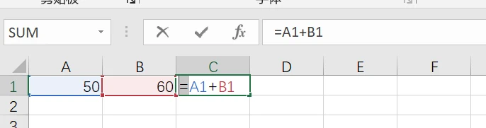
Functions are like tools that Excel has already prepared for you; each has its own name, followed by a pair of parentheses, inside which you placeParameters—That is, the data this function will process. After you finish typing and press Enter, Excel will calculate the result and display it in the cell, while the original formula remains in the formula bar above. If you click on that cell, you can see how the result was calculated by looking at the formula bar.
The best thing about formulas is that they update automatically as the data changes: if you change the source values, the results update automatically—that’s what makes them more flexible than a calculator. You can use arithmetic operators like addition, subtraction, multiplication, and division in formulas. Excel evaluates them according to mathematical order of operations; if you want to change the order, just add parentheses—the values inside the parentheses are calculated first.
Use a region to select a single grid cell
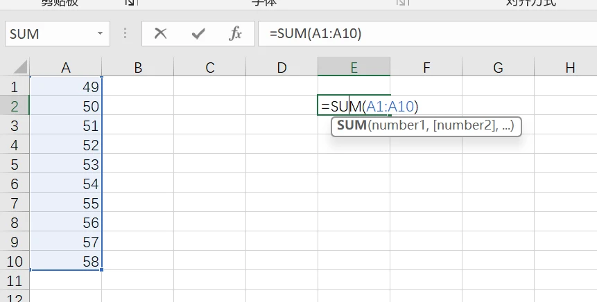
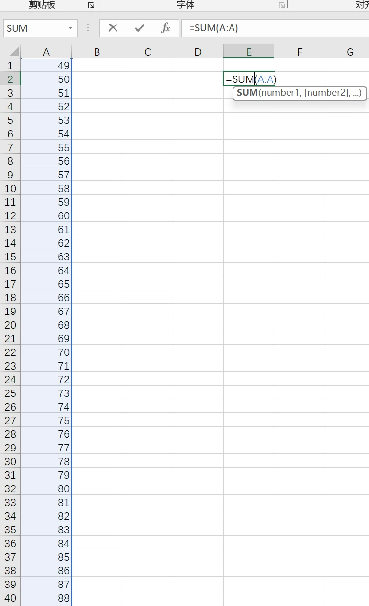
RegionIt refers to an entire range of cells—it can be a row, a column, or a block. To specify it, place a colon between the two cell addresses:
- A1:A10 refers to the range of data from A1 to A10:
- A: "A" refers to the entire column of data labeled "A":
- 1:1 represents all data in row 1:

Functions work especially well with ranges. SUM adds up the numbers within a range, AVERAGE calculates the average, and COUNT counts the number of values in a range. Using ranges in formulas is much shorter and clearer than listing cells one by one, and it makes it easier to change the range later. When you select a range, Excel highlights it with a colored border to help you verify that the range is correct; however, when you drag a formula down, the range shifts along with it, so you’ll need to make sure it hasn’t moved out of place.
Use $A$1 to lock the cell
QuoteThis is the cell address specified in the formula, which tells Excel where to retrieve the data. By default, it is a “relative reference”: when you drag the formula down, the row number increases automatically; when you drag it to the right, the column number increases automatically.
If you don't want it to move, just add a to the front of each column letter and row number. $。$A$1 This is an absolute reference; both the column and row are fixed, always pointing to that specific point.$A1 Lock only the columns; the rows can still change;A$1 Lock only the row; the column can still change—these two are called mixed references.Press F4 to toggle between these styles., Press a few more times to see it $ Running.
Absolute references are best suited for fixed values: Place that fixed number in its own cell, and use an absolute reference in the formula to point to it. That way, when you copy the formula, it won’t reference the wrong cell, and you’ll avoid a lot of pitfalls.
Understanding #N/A, #VALUE!, and #DIV/0!
Different error values have different meanings.
#N/A indicates that the item was not found; search functions return this error when no results are found.
#VALUE! indicates an invalid data type; the formula requires a number, but you entered text, so it returns this error.
#DIV/0! indicates division by zero; the divisor cannot be 0. Excel returns this error when it cannot perform the calculation.
When you see an error value, the general troubleshooting sequence is to first check the formula itself, then verify that the references are correct, and finally check whether there are any issues with the data format.
Common Questions for Beginners on Excel Formulas
Do Excel formulas have to start with an equals sign?
You must use the equals sign.=Introduction. Excel does not have a feature that automatically recognizes formulas; the only rule for determining whether a formula is present is that the cell content must begin with an equals sign for the system to recognize it as aExcel Formulasand perform calculations and evaluations; if no equals sign is included, Excel will display the input—whether it’s a function or an expression—as plain text and will not perform any calculations. In very rare cases, you can start with a plus or minus sign, but the standard, proper, and common practice isIt must begin with an equals sign.。
Can an Excel formula reference a data range that spans multiple worksheets?
Absolutely. Excel formulas support cross-worksheet data references; the basic syntax isWorksheet name + exclamation point! + cell/range address. For example, to reference cell A1 in the "Sheet2" worksheet, the formula would be =Sheet2!A1; If a worksheet name contains spaces or special characters, it must be enclosed in single quotes, for example ='Sales Data'!A2...allowing you to easily perform linked calculations across multiple tables.
What is the key difference between $A$1 and A1 in Excel formulas?
The difference between the two is thatCell Lock Status, which directly affects the formula drag-and-fill functionality.A1These are relative references; when you drag the formula, the row numbers and column labels will automatically shift to match the cell's new position;$A$1These are absolute references; the dollar sign $ locks both the column and the row, so no matter how you drag the formula to fill it in, the referenced cell positions always remain fixed. In addition, there are mixed references such as $A1 (lock the column but not the row) and A$1 (lock the row but not the column), which are core techniques for batch calculations in Excel formulas.
How do I replace the error value "#N/A" in an Excel formula with a blank cell?
#N/A is the most common "no match found" error in Excel formulas, indicating that the formula cannot find or match the corresponding data. You can useIFERROR Function或IFNA FunctionConvert error values to blank cells. IFERROR offers greater compatibility and can catch all formula errors. Syntax:=IFERROR(original formula, ""); IFNA specifically targets the #N/A error and does not suppress other error messages. Syntax:=IFNA(original_formula, ""), Just choose the one that suits your needs.
How can I prevent the "#DIV/0!" division-by-zero error from occurring in Excel formulas?
#DIV/0! is an Excel formula-specific error indicating division by zero. It occurs when the divisor in a division operation within a formula is blank or equal to 0. To resolve this, first useIF Function + Conditional LogicTo avoid invalid calculations, perform the operation only when the divisor is not equal to 0; if it is equal to 0, return a blank result or a specified prompt. General formula template:=IF(Divisor_Cell = 0, "", Dividend / Divisor)... This completely eliminates division-by-zero errors and makes the table look neater.
Do error values generated by Excel formulas need to be deleted or corrected?
There is no need to delete or modify them immediately. Various error values in Excel formulas (such as #N/A, #DIV/0!, #VALUE!, etc.) are essentiallyExcel Error Messages... Its purpose is to proactively highlight formula errors, data anomalies, parameter errors, and other issues, making it easier for us to troubleshoot problems such as incorrect formulas, missing data, and flawed calculation logic. We recommend first identifying and correcting formula errors based on the error values and organizing the source data. Once you have confirmed that the data and logic are correct, you can use a function to hide the error values and replace them with blanks.
Are function names in Excel formulas case-sensitive?
Function names in Excel formulas are not case-sensitive. Whether you type "if" or "vlookup" in lowercase, or "IF" or "VLOOKUP" in uppercase, Excel will automatically convert them to uppercase when you press Enter, and this will not affect the formula's results. However, when writing Excel formulas, it is recommended that you use a consistent case style to make them easier to read and check.
Does Excel support manual recalculation of formulas? What should I keep in mind when using F9?
Supports manual recalculation of Excel formulas; the F9 shortcut key forces a refresh of all formula calculations across all worksheets. Important note: If you select a cell and then press F9, the formula in that cell will be permanently replaced with the calculated static value, and the original formula will be lost and cannot be recovered. Therefore, do not select a formula cell when using F9; use it only to refresh calculations across the entire workbook.
Finally
Start with an equals sign, retrieve data from a range, use references to specify cell locations, and use error values to troubleshoot. Practice often, make corrections, and double-check your work—you’ll get the hang of it before you know it. The next time you open Excel, click a cell and start by typing an equals sign—and your first formula is done.